R Session: Linear Regression
One variable
First we need to load some libraries to access some datasets that we will be using.
library(MASS)
library(ISLR)
One of the datsets is the Boston data:
names(Boston)## [1] "crim" "zn" "indus" "chas" "nox" "rm" "age"
## [8] "dis" "rad" "tax" "ptratio" "black" "lstat" "medv"These are housing values for the suburbs of Boston. “medv” is the median value of owner occupied houses in Boston, while “lstat” is the lower status of the population in percentage. If we plot “medv” and “lstat”, we get the following plot.
plot(medv~lstat, Boston)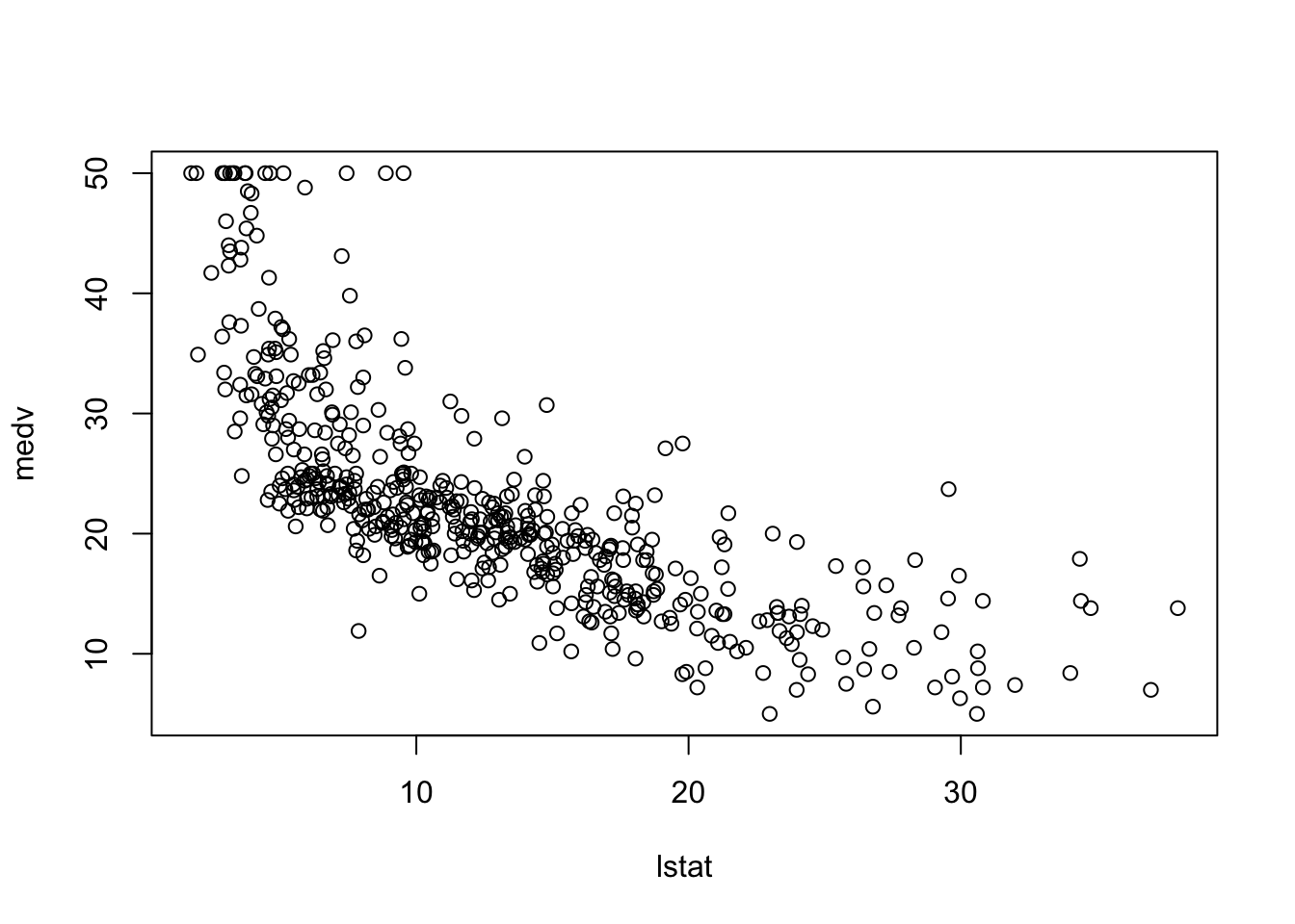
As the lower status in the region increases, we see a drop in the median housing values. If we fit a linear model to this model,
fit1 <- lm(medv~lstat, data = Boston)
fit1
##
## Call:
## lm(formula = medv ~ lstat, data = Boston)
##
## Coefficients:
## (Intercept) lstat
## 34.55 -0.95We see that the coefficient for slope is negative. To get a more detailed view of the model we can use the summary command.
summary(fit1)##
## Call:
## lm(formula = medv ~ lstat, data = Boston)
##
## Residuals:
## Min 1Q Median 3Q Max
## -15.168 -3.990 -1.318 2.034 24.500
##
## Coefficients:
## Estimate Std. Error t value Pr(>|t|)
## (Intercept) 34.55384 0.56263 61.41 <2e-16 ***
## lstat -0.95005 0.03873 -24.53 <2e-16 ***
## ---
## Signif. codes: 0 '***' 0.001 '**' 0.01 '*' 0.05 '.' 0.1 ' ' 1
##
## Residual standard error: 6.216 on 504 degrees of freedom
## Multiple R-squared: 0.5441, Adjusted R-squared: 0.5432
## F-statistic: 601.6 on 1 and 504 DF, p-value: < 2.2e-16To plot this linear model on to the plot, use thie following command:
plot(medv~lstat, Boston)
abline(fit1, col = "red")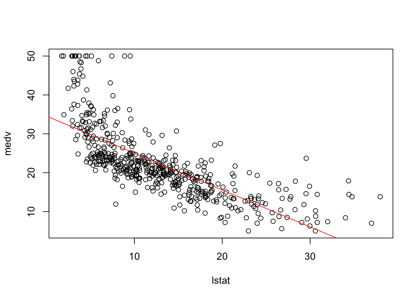
To find the confidence intervals for the coefficients of the linear model:
confint(fit1)## 2.5 % 97.5 %
## (Intercept) 33.448457 35.6592247
## lstat -1.026148 -0.8739505Notice how the confidence interval for “lstat” or the slope does not contain 0. This means that we reject the null hypothesis that there is no relationship between the variables. we say, there is some relationship. This is the 95% confidence interval.
We can predict the value of the response variable at any point along the predictor variable axis. This can be done by using predict. We can also ask R to give the confidence intervals for these predictions.
predict(fit1, data.frame(lstat=c(5,10,15)), interval = "confidence")## fit lwr upr
## 1 29.80359 29.00741 30.59978
## 2 25.05335 24.47413 25.63256
## 3 20.30310 19.73159 20.87461Multiple Linear Regression
We can use the same commands to fit using multiple predictors.
fit2 = lm(medv~lstat+age, data = Boston)
summary(fit2)
##
## Call:
## lm(formula = medv ~ lstat + age, data = Boston)
##
## Residuals:
## Min 1Q Median 3Q Max
## -15.981 -3.978 -1.283 1.968 23.158
##
## Coefficients:
## Estimate Std. Error t value Pr(>|t|)
## (Intercept) 33.22276 0.73085 45.458 < 2e-16 ***
## lstat -1.03207 0.04819 -21.416 < 2e-16 ***
## age 0.03454 0.01223 2.826 0.00491 **
## ---
## Signif. codes: 0 '***' 0.001 '**' 0.01 '*' 0.05 '.' 0.1 ' ' 1
##
## Residual standard error: 6.173 on 503 degrees of freedom
## Multiple R-squared: 0.5513, Adjusted R-squared: 0.5495
## F-statistic: 309 on 2 and 503 DF, p-value: < 2.2e-16fit3 = lm(medv~., data = Boston)
summary(fit3)##
## Call:
## lm(formula = medv ~ ., data = Boston)
##
## Residuals:
## Min 1Q Median 3Q Max
## -15.595 -2.730 -0.518 1.777 26.199
##
## Coefficients:
## Estimate Std. Error t value Pr(>|t|)
## (Intercept) 3.646e+01 5.103e+00 7.144 3.28e-12 ***
## crim -1.080e-01 3.286e-02 -3.287 0.001087 **
## zn 4.642e-02 1.373e-02 3.382 0.000778 ***
## indus 2.056e-02 6.150e-02 0.334 0.738288
## chas 2.687e+00 8.616e-01 3.118 0.001925 **
## nox -1.777e+01 3.820e+00 -4.651 4.25e-06 ***
## rm 3.810e+00 4.179e-01 9.116 < 2e-16 ***
## age 6.922e-04 1.321e-02 0.052 0.958229
## dis -1.476e+00 1.995e-01 -7.398 6.01e-13 ***
## rad 3.060e-01 6.635e-02 4.613 5.07e-06 ***
## tax -1.233e-02 3.760e-03 -3.280 0.001112 **
## ptratio -9.527e-01 1.308e-01 -7.283 1.31e-12 ***
## black 9.312e-03 2.686e-03 3.467 0.000573 ***
## lstat -5.248e-01 5.072e-02 -10.347 < 2e-16 ***
## ---
## Signif. codes: 0 '***' 0.001 '**' 0.01 '*' 0.05 '.' 0.1 ' ' 1
##
## Residual standard error: 4.745 on 492 degrees of freedom
## Multiple R-squared: 0.7406, Adjusted R-squared: 0.7338
## F-statistic: 108.1 on 13 and 492 DF, p-value: < 2.2e-16Here fit2 is the model using 2 predictors “lstat” and “age”. “age” is the proportion of owner occupied units built prior to 1940 in each region. fit3 is the model using every other variable in the dataset as predictors.
Notice how in fit2, “age” is a significant predictor but in fit3, “age” is no longer significant (check p-values). What that means is there are lot of other predictors that are correlated with “age” in whose presence, it is no longer significant.
We can plot the results of fit3. R normally gives us four different plots when we do this all of which are useful in determining the accuracy of the model.
par(mfrow = c(2,2))
plot(fit3)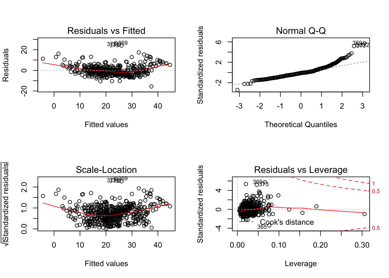
The first plot gives us a look at the residuals versus the fitted values. We can check for non-linearities in this figure. By the curve in the red line we can see that the residuals are not capturing the values well. There is some non-linearity.
The second plot tells us whether our assumption of normal distribution of the residuals is correct or not.
The third plot is the square root of the standardized residuals versus the fitted values. This gives us an idea of whether the variance changes with the mean or the fit. This is called heteroscedasticity. .
If we find that some variables are not significant predictors, we can remove these variables from the fitted model using the update command. Here we remove “age” and “indus” from the fitted model. Nothing on the left side of the “~” means we use the same response. We can use minus sign to remove the required variables.
fit4 = update(fit3, ~.-age-indus)
summary(fit4)
##
## Call:
## lm(formula = medv ~ crim + zn + chas + nox + rm + dis + rad +
## tax + ptratio + black + lstat, data = Boston)
##
## Residuals:
## Min 1Q Median 3Q Max
## -15.5984 -2.7386 -0.5046 1.7273 26.2373
##
## Coefficients:
## Estimate Std. Error t value Pr(>|t|)
## (Intercept) 36.341145 5.067492 7.171 2.73e-12 ***
## crim -0.108413 0.032779 -3.307 0.001010 **
## zn 0.045845 0.013523 3.390 0.000754 ***
## chas 2.718716 0.854240 3.183 0.001551 **
## nox -17.376023 3.535243 -4.915 1.21e-06 ***
## rm 3.801579 0.406316 9.356 < 2e-16 ***
## dis -1.492711 0.185731 -8.037 6.84e-15 ***
## rad 0.299608 0.063402 4.726 3.00e-06 ***
## tax -0.011778 0.003372 -3.493 0.000521 ***
## ptratio -0.946525 0.129066 -7.334 9.24e-13 ***
## black 0.009291 0.002674 3.475 0.000557 ***
## lstat -0.522553 0.047424 -11.019 < 2e-16 ***
## ---
## Signif. codes: 0 '***' 0.001 '**' 0.01 '*' 0.05 '.' 0.1 ' ' 1
##
## Residual standard error: 4.736 on 494 degrees of freedom
## Multiple R-squared: 0.7406, Adjusted R-squared: 0.7348
## F-statistic: 128.2 on 11 and 494 DF, p-value: < 2.2e-16Now everything in the model are somewhat significant.
Non-linearities and interactions
Interactiosn between two of the predictors can be included in the model by using an asterisk (*) symbol in the command:
fit5 = lm(medv~lstat*age, data = Boston)
summary(fit5)
##
## Call:
## lm(formula = medv ~ lstat * age, data = Boston)
##
## Residuals:
## Min 1Q Median 3Q Max
## -15.806 -4.045 -1.333 2.085 27.552
##
## Coefficients:
## Estimate Std. Error t value Pr(>|t|)
## (Intercept) 36.0885359 1.4698355 24.553 < 2e-16 ***
## lstat -1.3921168 0.1674555 -8.313 8.78e-16 ***
## age -0.0007209 0.0198792 -0.036 0.9711
## lstat:age 0.0041560 0.0018518 2.244 0.0252 *
## ---
## Signif. codes: 0 '***' 0.001 '**' 0.01 '*' 0.05 '.' 0.1 ' ' 1
##
## Residual standard error: 6.149 on 502 degrees of freedom
## Multiple R-squared: 0.5557, Adjusted R-squared: 0.5531
## F-statistic: 209.3 on 3 and 502 DF, p-value: < 2.2e-16This command includes the variables by themselves as well as the interaction term between the variables in the model. While the main effect of “age” by itself is not significant here, the interaction is somewhat significant.
Now, to include a quadratic term in the linear regression model, we have to protect the quadratic term with an “I” which stands for identity.
fit6 = lm(medv~lstat + I(lstat^2), data = Boston); summary(fit6)##
## Call:
## lm(formula = medv ~ lstat + I(lstat^2), data = Boston)
##
## Residuals:
## Min 1Q Median 3Q Max
## -15.2834 -3.8313 -0.5295 2.3095 25.4148
##
## Coefficients:
## Estimate Std. Error t value Pr(>|t|)
## (Intercept) 42.862007 0.872084 49.15 <2e-16 ***
## lstat -2.332821 0.123803 -18.84 <2e-16 ***
## I(lstat^2) 0.043547 0.003745 11.63 <2e-16 ***
## ---
## Signif. codes: 0 '***' 0.001 '**' 0.01 '*' 0.05 '.' 0.1 ' ' 1
##
## Residual standard error: 5.524 on 503 degrees of freedom
## Multiple R-squared: 0.6407, Adjusted R-squared: 0.6393
## F-statistic: 448.5 on 2 and 503 DF, p-value: < 2.2e-16par(mfrow=c(1,1))
plot(medv~lstat, data = Boston)
points(Boston$lstat, fitted(fit6), col = "red", pch = 20)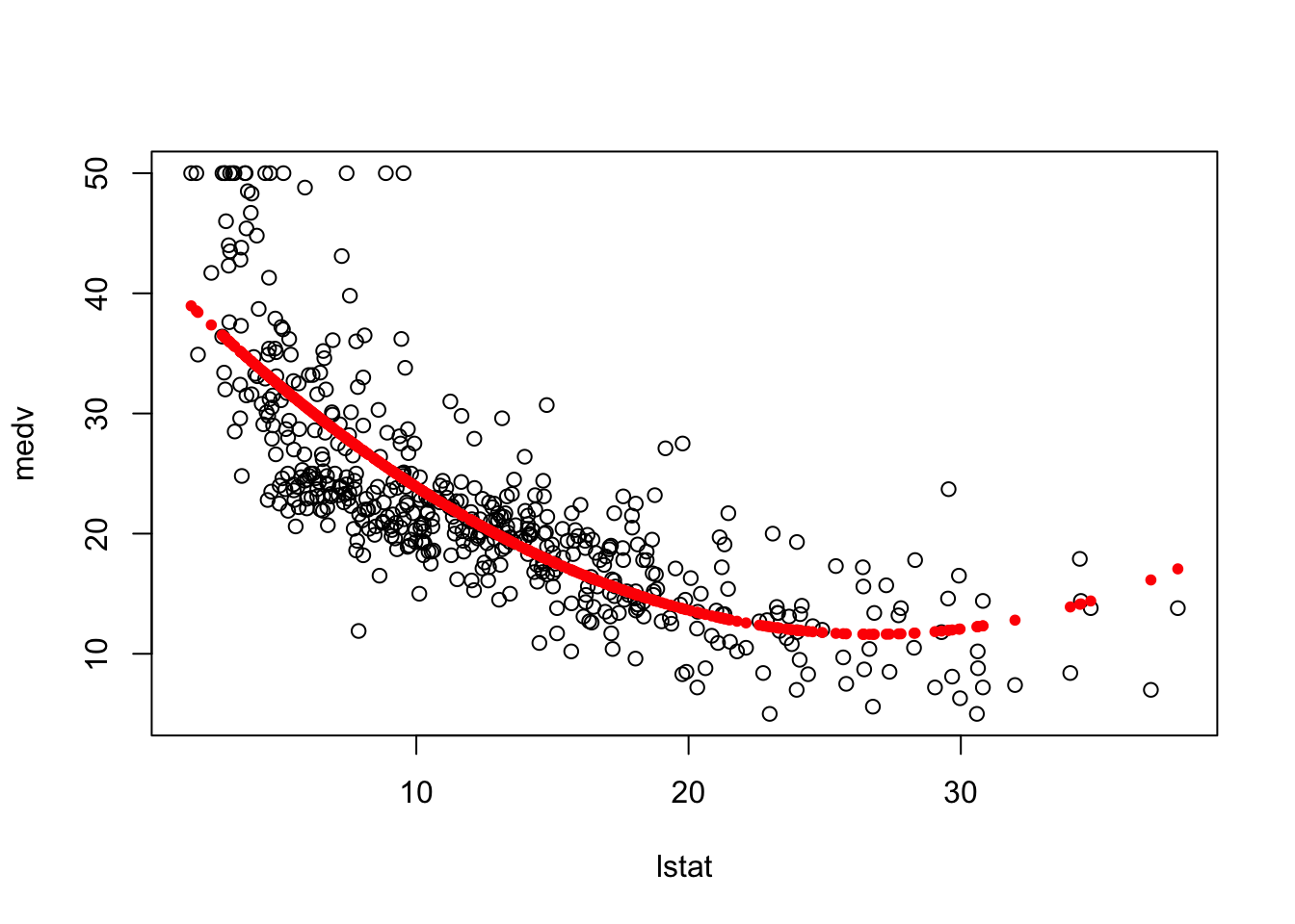
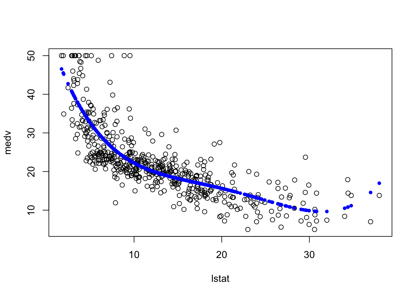
Now, what if we fit a polynomial function of degree 4 of the “lstat” variable. You can see how this is trying to overfit the data.
fit7 = lm(Boston$medv~poly(Boston$lstat,4))
plot(medv~lstat, data = Boston)
points(Boston$lstat, fitted(fit7), col = "blue", pch = 20)